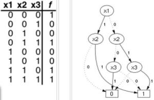
A binary decision diagram (BDD) or branching program, like a negation normal form (NNF) or a propositional directed acyclic graph (PDAG), is a data structure that is used to represent a Boolean function. On a more abstract level, BDDs can be considered as a compressed representation of sets or relations. Unlike other compressed representations, operations are performed directly on the compressed representation, i.e. without decompression.
A Boolean function can be represented as a rooted, directed, acyclic graph, which consists of decision nodes and two terminal nodes called 0-terminal and 1-terminal. Each decision node is labeled by a Boolean variable and has two child nodes called low child and high child. The edge from a node to a low (high) child represents an assignment of the variable to 0 (1). Such a BDD is called ‘ordered’ if different variables appear in the same order on all paths from the root. A BDD is said to be ‘reduced’ if the following two rules have been applied to its graph:
- Merge any isomorphic subgraphs.
- Eliminate any node whose two children are isomorphic.
In popular usage, the term BDD almost always refers to Reduced Ordered Binary Decision Diagram (ROBDD in the literature, used when the ordering and reduction aspects need to be emphasized). The advantage of an ROBDD is that it is canonical (unique) for a particular functionality.[citation needed] This property makes it useful in functional equivalence checking and other operations like functional technology mapping.
Below an example for a function f with three variables:
BDDs are useful for modeling software logic. By using them it is possible to evaluate test coverage and to generate tests for the program, bottom-up.
Symbolic Analysis and BDDs
For the reductionist implementation for Symbolic Analysis, there is only one global method for AHOs. It is the run-method intended for simulating each AHO atom.
It is rather easy to write another method to generate all possible paths for each AHO, because all branches happen in a path Clause (see book Symbolic Analysis). Lets our new method be bdd. We have a program P with the contents X1 • X2 • X3. After making an atomistic model, we have a model M, where the start element M0 is a model element with the contents meta(set([X1, X2, X3])). When we call M:bdd, then it call successively X1:bdd, X2:bdd and X3:bdd. Each of them returns a subtree as the clause formalism. In the main level the whole tree will be collected.
Summary: BDD can be seen as a small easy subset of simulation. BDD can be either static or partially dynamic, using method invokations as far as possible.
Some links:
- BDDs at Wiki: http://en.wikipedia.org/wiki/Binary_decision_diagram


 Formulation methodology
Leave a comment
Comments feed for this article